

Model Quantisation for Edge AI: Int8, Pruning and Distillation
Model quantisation for edge AI: zero points, calibration, int8-only maths, PTQ vs QAT, structured pruning and distillation, with numpy demos and LiteRT code.
Imagine you are flying from Indore to Bengaluru with only a 7 kg cabin bag, and your wardrobe weighs 30 kg. You don't cut every shirt in half. You leave out the clothes you never wear, roll the rest tightly, and pack one versatile jacket instead of three.
A trained neural network faces the same trip: built on a workstation with gigabytes of memory, it must now fit a robot's small board.
What is model quantisation for the edge?
Map the trip onto the model. Rolling clothes tightly is quantisation: the same weights, stored in fewer bits. Leaving out unworn clothes is pruning. One versatile jacket replacing three is distillation: a smaller model that learns to do what a bigger one did. The 7 kg limit is your device's flash, RAM and latency budget.
Model quantisation is the process of representing a neural network's weights and activations with low-precision integers, typically int8, plus a scale and zero point per tensor or channel, so the model needs less memory and can run on fast, low-power integer hardware.
Edge AI explained showed symmetric int8 weights and per-channel scales. This article goes deeper: activations, calibration, integer-only arithmetic, pruning and distillation.
How does affine quantisation work?
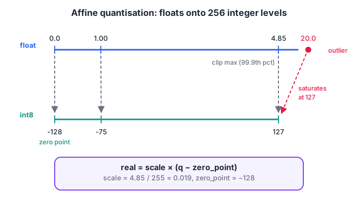
The scale sets the step between integer levels; the zero point says which integer stands for real 0.0.
Every quantised tensor uses one formula:
real_value = scale × (integer − zero_point)
The scale is the size of one integer step in real units. The zero point is the integer that represents exactly 0.0. Weights are roughly centred on zero, so they usually use a symmetric scheme with the zero point fixed at 0.
Activations after a ReLU are never negative, so a symmetric scheme would waste the whole negative half of the int8 range. Affine (asymmetric) quantisation fixes that by shifting the zero point, here to −128, so all 256 levels cover the values that actually occur.
Calibration: choosing the range
Weights are known after training, but activation ranges depend on the inputs. Calibration runs a few hundred realistic samples through the model and records each activation's range. The choice that matters is how to handle rare extreme values.
import numpy as np
rng = np.random.default_rng(3)
# ReLU outputs: all >= 0, mostly small, a few rare spikes
act = np.maximum(rng.normal(0.8, 1.0, 20000), 0).astype(np.float32)
act[:20] = rng.uniform(15, 25, 20)            # 0.1% outliers

def affine_params(lo, hi):                    # map [lo, hi] onto int8 [-128, 127]
    scale = (hi - lo) / 255
    zero_point = int(round(-128 - lo / scale))
    return scale, zero_point

def fake_quant(x, scale, zp):
    q = np.clip(np.round(x / scale) + zp, -128, 127)
    return (q - zp) * scale

sym_scale = np.abs(act).max() / 127           # symmetric: wastes the negative half
tests = {
    "symmetric, min-max": (sym_scale, 0),
    "affine, min-max": affine_params(act.min(), act.max()),
    "affine, 99.9th pct": affine_params(0.0, np.percentile(act, 99.9)),
}
for name, (s, zp) in tests.items():
    err = np.abs(act - fake_quant(act, s, zp))
    print(f"{name:19s} scale={s:.4f} zp={zp:4d}  typical err={err[20:].mean():.4f}"
          f"  outlier err={err[:20].mean():.2f}")
Affine quantisation halves the error compared with symmetric, for free. Clipping at the 99.9th percentile cuts the error on typical values by another five times, because 20 rare spikes no longer stretch the scale, but those spikes now saturate.
Whether that is acceptable depends on the layer, so toolchains offer min-max, percentile and entropy calibration to compare on a validation set.
Quick check
Why do ReLU activations usually use affine (asymmetric) quantisation?
Shifting the zero point lets all 256 levels cover the 0-to-max range that actually occurs.
What does integer-only inference look like?
On a microcontroller or NPU, the whole layer runs in integers. Each int8 input is multiplied by an int8 weight, and the products are summed in an int32 accumulator so they cannot overflow. The result is then requantised to int8 for the next layer, using a precomputed fixed-point multiplier and a bit shift instead of a float division.
import numpy as np
rng = np.random.default_rng(5)
x = np.maximum(rng.normal(0.5, 1, 64), 0).astype(np.float32)   # input activations
W = rng.normal(0, 0.1, (64, 16)).astype(np.float32)            # layer weights
y = x @ W                                                      # float reference

s_x, z_x = x.max() / 255, -128                 # affine int8 input
s_w = np.abs(W).max(axis=0) / 127              # symmetric per-channel weights
s_y = (y.max() - y.min()) / 255               # affine int8 output
z_y = int(round(-128 - y.min() / s_y))
q_x = np.clip(np.round(x / s_x) + z_x, -128, 127).astype(np.int8)
q_w = np.round(W / s_w).astype(np.int8)

# Integer-only: int8 x int8 products summed in an int32 accumulator
acc = (q_x.astype(np.int32) - z_x) @ q_w.astype(np.int32)
M = s_x * s_w / s_y                            # real multiplier per channel
shift = 31 - np.ceil(np.log2(M)).astype(np.int64)
M0 = np.round(M * 2.0 ** shift).astype(np.int64)   # fixed-point int32 multiplier
q_y = np.clip(((acc * M0) >> shift) + z_y, -128, 127).astype(np.int8)

y_back = (q_y.astype(np.float32) - z_y) * s_y
print("accumulator dtype:", acc.dtype, " max |acc|:", np.abs(acc).max())
print("fixed-point multipliers (first 3):", M0[:3], "shifts:", shift[:3])
print("float  :", np.round(y[:5], 3))
print("int8   :", np.round(y_back[:5], 3))
print(f"max abs error {np.abs(y - y_back).max():.4f}  (output step = {s_y:.4f})")
The int32 accumulator holds values in the tens of thousands, which would overflow int8 or int16 immediately. The requantisation multiplier is an ordinary integer, so no floating-point unit is needed, and the final outputs land within about two output steps of the float result.
This is essentially what the int8 kernels in LiteRT for Microcontrollers and CMSIS-NN do, though real kernels use rounding shifts for a little more accuracy.
Post-training quantisation vs quantisation-aware training
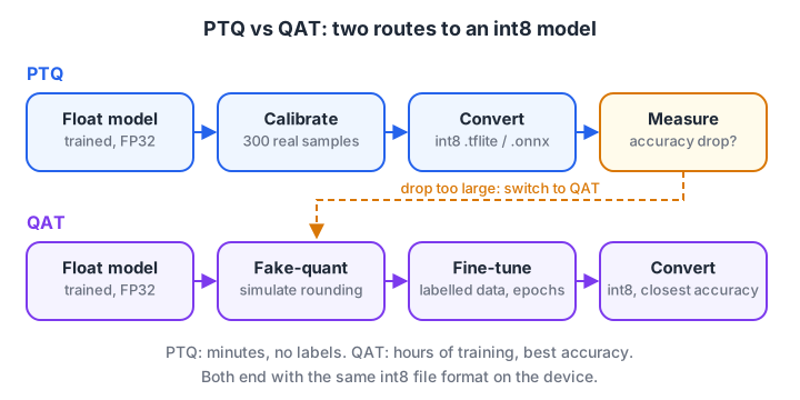
Try PTQ first. Use QAT only when the accuracy drop after PTQ is too large.
| Post-training quantisation (PTQ) | Quantisation-aware training (QAT) | |
|---|---|---|
| When it happens | After training, during conversion | During extra fine-tuning epochs |
| Data needed | A few hundred unlabelled calibration samples | The labelled training set |
| Effort | Minutes | Hours to days of training |
| Typical accuracy | Fine for most CNNs; may drop for small or sensitive models | Usually closest to the float model |
| How | Converter options in LiteRT, ONNX Runtime, OpenVINO NNCF | Fake-quantisation layers that simulate rounding while training |
A practical rule: run PTQ, measure accuracy on your validation set, and if the drop is more than you can accept, first try per-channel weights, percentile calibration or keeping the first and last layers at higher precision. Move to QAT only after that.
Large language models use a different recipe, usually 4-bit weight-only quantisation with float activations, because they are limited by memory bandwidth. That is covered in LLM inference optimisation.
How do pruning and distillation shrink a model?
Structured pruning beats unstructured on real hardware
Pruning removes parameters that contribute little. Unstructured pruning zeroes individual weights anywhere in a matrix. Structured pruning removes whole neurons, filters or channels, so the matrices actually get smaller.
import numpy as np
rng = np.random.default_rng(11)
# Two-layer network: 128 inputs -> 256 hidden (ReLU) -> 10 outputs
W1 = rng.normal(0, 0.1, (128, 256)) * rng.uniform(0.05, 1.5, 256)  # some neurons weak
W2 = rng.normal(0, 0.1, (256, 10))
X = rng.normal(0, 1, (500, 128))
forward = lambda X, A, B: np.maximum(X @ A, 0) @ B
ref = forward(X, W1, W2)

# Unstructured: zero the 50% smallest weights. Shapes do not change.
cut = np.quantile(np.abs(W1), 0.5)
W1_u = np.where(np.abs(W1) < cut, 0, W1)
# Structured: drop the 128 hidden neurons with the smallest L1 norm.
keep = np.argsort(np.abs(W1).sum(axis=0))[128:]
W1_s, W2_s = W1[:, keep], W2[keep, :]

for name, A, B in [("original", W1, W2), ("unstructured 50%", W1_u, W2),
                   ("structured 50%", W1_s, W2_s)]:
    out = forward(X, A, B)
    agree = (out.argmax(1) == ref.argmax(1)).mean()
    dense_macs = A.shape[0] * A.shape[1] + B.shape[0] * B.shape[1]
    print(f"{name:17s} W1 shape {str(A.shape):10s} nonzeros {np.count_nonzero(A):6d}"
          f"  dense MACs {dense_macs:6d}  same top class {agree:.0%}")
Unstructured pruning halves the non-zero weights and keeps 87% of top-class answers, but the matrix shape and the dense MAC count do not change, so a normal CPU or NPU runs exactly as many multiplications as before.
Structured pruning halves the real work. It also disturbs the outputs more (66% agreement here), which is why it is always followed by fine-tuning. Only hardware or libraries with sparse support gain speed from unstructured zeros.
Knowledge distillation: a small student learns from a big teacher
Distillation trains a small student model to match a large teacher model's output probabilities, not just the hard labels. The trick is a temperature T that softens the teacher's probabilities so the student can see which wrong answers are "nearly right".
import numpy as np
def softmax(z, T=1.0):
    e = np.exp((z - z.max()) / T)
    return e / e.sum()

classes = ["person", "chair", "dog", "box"]
teacher_logits = np.array([6.0, 3.5, 2.8, -1.0])    # big model's raw scores
for T in (1, 4):
    p = softmax(teacher_logits, T)
    print(f"T={T}: " + "  ".join(f"{c} {v:.3f}" for c, v in zip(classes, p)))

# Distillation loss for one example: hard label + softened teacher (T=4)
student_logits = np.array([4.0, 1.0, 2.5, 0.5])
T, alpha = 4.0, 0.7
p_t, p_s = softmax(teacher_logits, T), softmax(student_logits, T)
kl = np.sum(p_t * np.log(p_t / p_s)) * T * T        # scaled by T^2, as is standard
ce = -np.log(softmax(student_logits)[0])            # true class = person
print(f"soft loss (KL x T^2) {kl:.3f}, hard loss (CE) {ce:.3f}, "
      f"total {alpha * kl + (1 - alpha) * ce:.3f}")
At T = 1 the teacher is 89% sure it sees a person, and the other classes look almost equally unlikely. At T = 4 you can see that it thinks "chair" and "dog" are much more plausible than "box".
That ranking is extra knowledge the student cannot get from a one-hot label. The loss mixes the soft term (scaled by T², as is standard) and the usual cross-entropy on the true label.
Quick check
Which pruning method reduces the number of multiplications on an ordinary CPU or NPU?
Removing whole channels makes the matrices smaller; scattered zeros keep the same dense shape.
Doing it with real toolchains
Here is full-integer PTQ for a Keras model with the TensorFlow converter, which produces LiteRT .tflite files. The representative dataset is your calibration set.
import numpy as np
import tensorflow as tf

model = tf.keras.models.load_model("obstacle_net.keras")
calib = np.load("robot_camera_calib.npy").astype(np.float32)   # e.g. 300 real frames

def representative_dataset():
    for frame in calib:
        yield [frame[np.newaxis, ...]]

converter = tf.lite.TFLiteConverter.from_keras_model(model)
converter.optimizations = [tf.lite.Optimize.DEFAULT]
converter.representative_dataset = representative_dataset
converter.target_spec.supported_ops = [tf.lite.OpsSet.TFLITE_BUILTINS_INT8]
converter.inference_input_type = tf.int8      # fully integer, for MCUs and NPUs
converter.inference_output_type = tf.int8
open("obstacle_net_int8.tflite", "wb").write(converter.convert())
ONNX Runtime has the same idea for .onnx models, with static quantisation in the QDQ format that most execution providers accept.
import numpy as np
from onnxruntime.quantization import (CalibrationDataReader, QuantFormat,
                                      QuantType, quantize_static)

class CameraFrames(CalibrationDataReader):
    def __init__(self, frames, input_name):
        self.it = iter([{input_name: f[np.newaxis]} for f in frames])
    def get_next(self):
        return next(self.it, None)

frames = np.load("robot_camera_calib.npy").astype(np.float32)   # NCHW frames
quantize_static("detector.onnx", "detector_int8.onnx",
                CameraFrames(frames, "images"),
                quant_format=QuantFormat.QDQ, per_channel=True,
                activation_type=QuantType.QInt8, weight_type=QuantType.QInt8)
For Intel CPUs, GPUs and NPUs, OpenVINO's NNCF library does the same job with nncf.quantize() and offers nncf.prune() for structured pruning (OpenVINO 2026.3 at the time of writing). Whatever the tool, measure accuracy and latency on the target board afterwards, as the edge AI hardware guide recommends.
For microcontrollers, the result then goes through the firmware steps in TinyML explained. Once the model is small enough, the next question is where each part of the robot's software should run, which edge-cloud robotics answers.
Common quantisation mistakes
- Calibrating with too few or unrealistic samples. Ranges come out wrong and accuracy collapses only on the robot.
- Forgetting the input pipeline. A fully int8 model expects quantised inputs with its own scale and zero point.
- Assuming every operator is supported. Layers left in float on an int8 NPU fall back to the CPU and can erase the gain.
Key takeaways
- Quantised tensors use
real = scale × (q − zero_point); weights are usually symmetric per channel, activations affine. - Calibration with realistic data sets activation ranges; percentile clipping trades rare outliers for precision.
- Integer kernels accumulate in int32 and requantise with a fixed-point multiplier.
- Try PTQ first and QAT only if the accuracy drop is too large.
- Structured pruning and distillation shrink the real compute; always fine-tune and re-measure.
FAQ
Does int8 quantisation reduce accuracy?
Usually a little. Many vision models lose under a percentage point with good calibration and per-channel weights, but small or unusual models can lose more. Always compare the quantised model against the float model on a validation set from your own device, and use quantisation-aware training if the drop is too large.
What is the difference between dynamic and static quantisation?
Dynamic quantisation stores weights as int8 but computes activation ranges at run time, so it needs no calibration data and suits CPUs running language models. Static quantisation fixes activation ranges in advance using calibration samples, which allows fully integer inference on microcontrollers and NPUs.
What is a zero point in quantisation?
The zero point is the integer that represents the real value 0.0. It lets an asymmetric range, such as 0 to 6 for ReLU6 outputs, use all 256 int8 levels. Symmetric weight quantisation fixes the zero point at 0, which keeps the integer maths simpler.
Should I prune or quantise first?
Usually prune and fine-tune first, then quantise, because quantisation ranges should be computed on the final weights. Distillation, if used, comes before both, since it produces the small model you then optimise. Measure accuracy after each step so you know which one costs what.
Where can I learn to deploy optimised models on robots in Indore?
Debugshala's robotics course at Old Palasia builds the base you need: Python, Arduino and ESP32, sensors, Raspberry Pi with a camera and ROS 2 basics, ending in a final project. Read about the Raspberry Pi and ROS 2 course modules at Debugshala, and book a free demo class. For model-side practice, attempt the coding quizzes on Debugshala Test.
From the team behind this site
Go further with the Robotics Course at Debugshala
These tutorials are written by Debugshala, a training and placement institute at Old Palasia, Indore. The classroom course adds live mentoring, real projects and interview preparation.
- Offline classes at Old Palasia, Indore
- Free demo class before you pay
- Non-IT, fresher and year-gap friendly
- Placement assistance
700+ students placed · 200+ hiring partners · 4.9★ Google rating
