

ROS 2 Navigation with Nav2: Costmaps, Planners and Controllers
How Nav2 navigates a robot in ROS 2 Jazzy: servers, behaviour trees, costmap inflation, planners, controllers, nav2_params.yaml and Python goal sending.
Think of a delivery rider in Indore taking an order from Sarafa to Bhawarkua. Before starting, the app shows a route on the city map. The rider does not follow it blindly, though: a cow in the lane, a parked tempo, a dug-up stretch of road, and the rider swerves, slows or waits, then rejoins the route.
If the lane is completely blocked, the rider backs out and the app finds another way. And the rider always knows roughly where they are, from landmarks and GPS, even when the map is slightly out of date.
That is the shape of robot navigation: a map, a sense of position, a long-range plan, short-range steering around surprises, and a plan B when stuck.
What is Nav2 in ROS 2?
Map the delivery onto a robot. The city map is a saved occupancy grid, like the one you build in robot localisation and SLAM. Knowing where you are is localisation, done by AMCL.
The app's route is the global plan, made by the planner. Swerving around the cow is the controller reacting on a local costmap. Backing out of a blocked lane is a recovery behaviour. And the app deciding when to reroute is the behaviour tree.
Nav2 is the open-source navigation framework for ROS 2 that moves a mobile robot from its current pose to a goal pose, using costmaps, pluggable path planners and controllers, localisation and recovery behaviours coordinated by a behaviour tree.
This lesson targets ROS 2 Jazzy with Gazebo Harmonic; Nav2 also has Lyrical binaries. It uses the simulated robot from robot simulation with Gazebo, which already publishes /scan, /odom and TF.
How does Nav2 work? The architecture
Nav2 is a group of ROS 2 servers, each with one job, and almost every algorithm inside them is a swappable plugin.
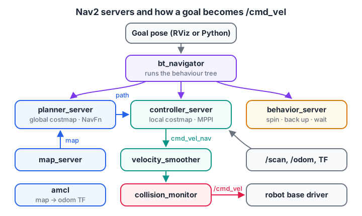
Goals go in at the top as actions; velocity commands come out at the bottom. Everything in between is a replaceable plugin.
| Server | Job | Jazzy default plugin |
|---|---|---|
| bt_navigator | Runs the behaviour tree that sequences planning, control and recovery | NavigateToPose, NavigateThroughPoses |
| planner_server | Computes a path from the robot to the goal on the global costmap | NavFn (Dijkstra, or A* if enabled) |
| controller_server | Follows the path, producing velocity commands at about 20 Hz | MPPI controller |
| smoother_server | Smooths jagged planned paths | Simple smoother |
| behavior_server | Recovery actions: spin, back up, drive on heading, wait | Spin, BackUp, Wait and others |
| velocity_smoother, collision_monitor | Limit acceleration; stop or slow if something is too close | — |
| map_server, amcl | Load the saved map; estimate the robot's pose on it | Particle filter |
The lifecycle manager starts the servers in order. The controller's output, cmd_vel_nav, passes through the velocity smoother and collision monitor before reaching /cmd_vel and your differential drive base.
What Nav2 needs from your robot
Nav2 assumes the standard REP 105 frame tree. If any link is missing, nothing moves.
- map → odom, from AMCL (or slam_toolbox when mapping).
- odom → base_link, from your odometry source, such as Gazebo's DiffDrive system.
- base_link → sensor frames, from robot_state_publisher and the URDF.
/scan(or a point cloud) and/odomtopics.- A base driver that obeys
/cmd_vel.
Quick check
Which Nav2 server turns the planned path into velocity commands?
The controller server runs the path-following plugin (MPPI by default in Jazzy) at about 20 Hz and outputs velocity commands.
Try Nav2 in simulation first
Nav2 ships a complete TurtleBot simulation, the quickest way to see every piece working before you configure your own robot.
sudo apt install ros-jazzy-navigation2 ros-jazzy-nav2-bringup ros-jazzy-nav2-minimal-tb*
source /opt/ros/jazzy/setup.bash
ros2 launch nav2_bringup tb3_simulation_launch.py headless:=False
Gazebo and RViz open together. Then:
- Click 2D Pose Estimate in RViz and drag an arrow where the robot is. AMCL needs this starting guess.
- Click Nav2 Goal and drag an arrow to the destination.
- Watch the global path appear and the robot drive around obstacles.
Drop a box in its way in Gazebo: the local costmap marks it and the controller steers around it.
What is a costmap and how does inflation work?
A costmap is a 2D grid, typically 5 cm per cell, holding costs from 0 to 255. Nav2 keeps a global costmap for planning and a 3 m by 3 m local costmap that rolls along with the robot for control.
| Cost value | Meaning |
|---|---|
| 0 | Free space |
| 1 to 252 | Near an obstacle; higher is closer |
| 253 | Inscribed: the robot's centre here means its body touches an obstacle |
| 254 | Lethal: an obstacle occupies this cell |
| 255 | Unknown, no information |
Costmaps are built from layers: the static layer copies the saved map, the obstacle layer marks lidar hits and clears free space, and the inflation layer spreads cost around obstacles.
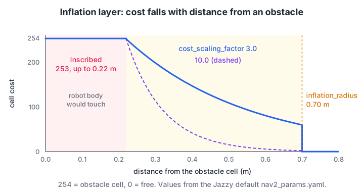
A low cost_scaling_factor keeps cost high further from obstacles, so the planner prefers the middle of corridors.
Inside the inscribed radius the cost is 253. Beyond it, Nav2's inflation layer uses 252 × exp(−cost_scaling_factor × (distance − inscribed_radius)), cut to zero past inflation_radius. This block uses the Jazzy defaults and a steeper alternative.
import math

INSCRIBED, LETHAL = 253, 254

def inflation_cost(dist, inscribed_r=0.22, inflation_r=0.70, scaling=3.0):
    if dist == 0:
        return LETHAL
    if dist <= inscribed_r:
        return INSCRIBED
    if dist > inflation_r:
        return 0
    return int((INSCRIBED - 1) * math.exp(-scaling * (dist - inscribed_r)))

print("distance m | scaling 3.0 | scaling 10.0")
for d in (0.0, 0.10, 0.22, 0.25, 0.30, 0.40, 0.50, 0.60, 0.70, 0.75):
    print(f"   {d:5.2f}   |    {inflation_cost(d):3d}      |    {inflation_cost(d, scaling=10.0):3d}")
With the default scaling of 3.0, a cell 0.5 m from a wall still costs 108, so the planner centres itself in corridors. With 10.0, the cost has almost vanished by 0.5 m, and paths cut close to walls.
Build an inflated costmap on a small grid
Here is the whole inflation layer applied to a 2.4 m by 1.4 m corridor at 10 cm per cell, with walls along the top and bottom and a box in the middle. Each character shows a cost band.
import numpy as np

res, H, W = 0.10, 14, 24
occ = np.zeros((H, W), bool)
occ[0, :] = occ[-1, :] = True              # top and bottom walls
occ[5:9, 11:13] = True                     # a box in the middle

obs = np.argwhere(occ)
rows, cols = np.indices((H, W))
cells = np.stack([rows.ravel(), cols.ravel()], axis=1)
dist = np.sqrt(((cells[:, None, :] - obs[None, :, :]) ** 2).sum(-1)).min(1).reshape(H, W) * res

inscribed, inflation, scaling = 0.10, 0.35, 3.0
cost = np.where(dist > inflation, 0, (252 * np.exp(-scaling * (dist - inscribed))).astype(int))
cost[dist <= inscribed] = 253
cost[occ] = 254

def symbol(c):
    return "#" if c == 254 else "x" if c == 253 else "+" if c > 150 else "." if c > 0 else " "
for r in range(H):
    print("".join(symbol(c) for c in cost[r]))
print("free cells:", int((cost == 0).sum()), "of", H * W)
# is lethal, x is inscribed, + is high cost and . is low cost. The blank lanes above and below the box are where a planner prefers to drive.
Quick check
A costmap cell has the value 253. What does it mean?
253 is the inscribed cost. 254 is lethal (an obstacle in the cell) and 255 means no information.
Planning and following a path
The planner searches the global costmap for the cheapest path, mixing distance with obstacle cost, using Dijkstra or A* style searches from path planning with A* and Dijkstra. Here it has two ways through a partition: a 20 cm gap on the direct line and a 60 cm doorway further away.
import heapq, numpy as np

H, W, res = 16, 16, 0.10
occ = np.zeros((H, W), bool); occ[[0, -1], :] = True; occ[:, 7:9] = True    # walls and a partition
occ[5:7, 7:9] = False                     # narrow gap, 0.2 m wide, on the direct line
occ[9:15, 7:9] = False                    # wide doorway, 0.6 m, further away
obs, cells = np.argwhere(occ), np.argwhere(np.ones((H, W)))
d = np.sqrt(((cells[:, None] - obs[None]) ** 2).sum(-1)).min(1).reshape(H, W) * res
cost = np.where(d > 0.4, 0, 252 * np.exp(-3.0 * (d - 0.05))).astype(int)
cost[occ] = 254

def plan(start, goal, weight):
    frontier, came, g = [(0, start)], {start: None}, {start: 0.0}
    while frontier and (cur := heapq.heappop(frontier)[1]) != goal:
        for nxt in ((cur[0] + 1, cur[1]), (cur[0] - 1, cur[1]), (cur[0], cur[1] + 1), (cur[0], cur[1] - 1)):
            if 0 <= nxt[0] < H and 0 <= nxt[1] < W and cost[nxt] < 253:
                new_g = g[cur] + 1 + weight * cost[nxt] / 252     # distance + obstacle cost
                if new_g < g.get(nxt, 1e9):
                    g[nxt], came[nxt] = new_g, cur
                    heapq.heappush(frontier, (new_g + abs(goal[0] - nxt[0]) + abs(goal[1] - nxt[1]), nxt))
    path, n = [], goal
    while n:
        path.append(n); n = came[n]
    return path[::-1]

for w in (0.0, 3.0, 10.0):
    p = plan((5, 0), (5, W - 1), w)
    gap = "narrow gap" if any(r < 8 for r, c in p if c == 7) else "wide doorway"
    print(f"weight {w:4}: {len(p) - 1} moves ({(len(p) - 1) * res:.1f} m) via the {gap}, "
          f"closest approach to a wall {min(d[c] for c in p):.2f} m")
With low weights the planner squeezes through the narrow gap, passing 10 cm from the walls. With a weight of 10 it accepts a path 1.2 m longer to go through the doorway with 30 cm of clearance. Nav2's planners expose the same trade-off; the Smac planners, for example, have a cost_penalty parameter.
A controller loop that follows the path
Every 50 ms, the controller looks at the path ahead and picks a linear and angular velocity. MPPI samples thousands of trajectories per cycle; the simpler Regulated Pure Pursuit steers towards a point a fixed distance ahead, as this loop does.
import math

path = [(0.1 * i, 0.4 * math.sin(0.1 * i)) for i in range(41)]   # a 4 m S-shaped path
x, y, th, dt = 0.0, -0.15, 0.0, 0.05                              # robot starts 15 cm off the path
LOOKAHEAD, V_MAX, W_MAX = 0.35, 0.3, 1.9

for step in range(400):
    if math.hypot(path[-1][0] - x, path[-1][1] - y) < 0.05:
        break
    near = min(range(len(path)), key=lambda i: math.hypot(path[i][0] - x, path[i][1] - y))
    tx, ty = next((p for p in path[near:] if math.hypot(p[0] - x, p[1] - y) >= LOOKAHEAD), path[-1])
    lx = math.cos(-th) * (tx - x) - math.sin(-th) * (ty - y)     # target in the robot frame
    ly = math.sin(-th) * (tx - x) + math.cos(-th) * (ty - y)
    curvature = 2 * ly / (lx ** 2 + ly ** 2)
    v = V_MAX
    w = max(-W_MAX, min(W_MAX, v * curvature))                    # this pair goes on /cmd_vel
    x += v * math.cos(th) * dt; y += v * math.sin(th) * dt; th += w * dt
    if step % 25 == 0:
        err = min(math.hypot(px - x, py - y) for px, py in path)
        print(f"t={step * dt:4.2f}s pos=({x:4.2f},{y:5.2f}) v={v:.2f} w={w:5.2f} off-path={err * 100:4.1f} cm")
print(f"goal reached at t={step * dt:.2f}s, final position ({x:.2f}, {y:.2f})")
The robot starts 15 cm off the path, converges over about four seconds, then tracks the curve within about 5 cm, cutting corners slightly because it aims 35 cm ahead. Real controllers also slow on sharp curves and check each command against the local costmap.
Configure Nav2 for your own robot
The usual approach is to copy the default parameter file and edit only what differs for your robot.
mkdir -p ~/ros2_ws/src/my_robot_description/config
cp $(ros2 pkg prefix --share nav2_bringup)/params/nav2_params.yaml \
   ~/ros2_ws/src/my_robot_description/config/nav2_params.yaml
For the 20 cm robot from earlier lessons, edit its size, inflation and speed limits. These are excerpts, not a complete file.
amcl:
  ros__parameters:
    base_frame_id: "base_footprint"
    scan_topic: scan

controller_server:
  ros__parameters:
    controller_frequency: 20.0
    FollowPath:
      plugin: "nav2_mppi_controller::MPPIController"
      motion_model: "DiffDrive"
      vx_max: 0.3          # slower than the 0.5 m/s default
      wz_max: 1.9

local_costmap:
  local_costmap:
    ros__parameters:
      robot_radius: 0.13   # half the diagonal of the 0.20 x 0.14 m body, plus margin
      inflation_layer:
        plugin: "nav2_costmap_2d::InflationLayer"
        cost_scaling_factor: 3.0
        inflation_radius: 0.45

global_costmap:
  global_costmap:
    ros__parameters:
      robot_radius: 0.13
      inflation_layer:
        plugin: "nav2_costmap_2d::InflationLayer"
        cost_scaling_factor: 3.0
        inflation_radius: 0.45

planner_server:
  ros__parameters:
    planner_plugins: ["GridBased"]
    GridBased:
      plugin: "nav2_navfn_planner::NavfnPlanner"
      tolerance: 0.5
      use_astar: false
      allow_unknown: true
Then start your simulation and bring up Nav2 with your map and parameters. Set slam:=True and leave out the map instead, if you want to map and navigate at the same time.
# Terminal 1: the Gazebo simulation from the previous lesson
ros2 launch my_robot_description sim.launch.py

# Terminal 2: Nav2 with a saved map and your parameters
ros2 launch nav2_bringup bringup_launch.py use_sim_time:=True \
  map:=$HOME/maps/lab_map.yaml \
  params_file:=$HOME/ros2_ws/src/my_robot_description/config/nav2_params.yaml

# Terminal 3: RViz with the Nav2 panels
ros2 launch nav2_bringup rviz_launch.py
Send goals from Python
The nav2_simple_commander package wraps Nav2's actions in a few Python calls, so an application can send goals without writing action clients by hand.
import rclpy
from geometry_msgs.msg import PoseStamped
from nav2_simple_commander.robot_navigator import BasicNavigator, TaskResult


def make_pose(nav, x, y):
    pose = PoseStamped()
    pose.header.frame_id = 'map'
    pose.header.stamp = nav.get_clock().now().to_msg()
    pose.pose.position.x, pose.pose.position.y = x, y
    pose.pose.orientation.w = 1.0
    return pose


def main():
    rclpy.init()
    nav = BasicNavigator()
    nav.setInitialPose(make_pose(nav, 0.0, 0.0))
    nav.waitUntilNav2Active()            # waits for AMCL and the servers

    nav.goToPose(make_pose(nav, 2.0, 1.0))
    while not nav.isTaskComplete():
        feedback = nav.getFeedback()
        if feedback:
            print(f'distance remaining: {feedback.distance_remaining:.2f} m')

    result = nav.getResult()
    print('arrived' if result == TaskResult.SUCCEEDED else f'navigation ended: {result}')
    nav.lifecycleShutdown()
    rclpy.shutdown()


if __name__ == '__main__':
    main()
goThroughPoses() and followWaypoints() work the same way for multi-stop routes, such as a robot visiting three classroom tables in turn.
Common Nav2 mistakes
- No initial pose. Until AMCL gets a 2D Pose Estimate or
setInitialPose, map → odom is missing. - Mixed
use_sim_time. Set it on every node in simulation, and on none with hardware. - A wrong robot radius. Too small clips corners; too large blocks doorways.
- Inflation radius smaller than the inscribed radius. Cost jumps from 253 to 0, and paths hug walls.
- Mismatched frame names. AMCL's
base_frame_idand the costmaps'robot_base_framemust exist in TF. - The base ignores
/cmd_vel. Runros2 topic echo /cmd_velduring a goal and check the message type.
The planner and controller blocks are graph search and geometry at heart, so practise graph-search and grid questions on Debugshala Test to keep those skills sharp.
Key takeaways
- Nav2 moves a robot to a goal pose using a planner, a controller, recoveries and a behaviour tree.
- It needs map → odom → base_link TF, a scan or point cloud, odometry and a base that obeys
/cmd_vel. - Costmaps hold 0 to 254 costs; inflation decays exponentially from the inscribed radius to the inflation radius.
- Jazzy's default bringup uses NavFn for planning and MPPI for control, all swappable in YAML.
- Start with
tb3_simulation_launch.py, then copy and editnav2_params.yamlfor your own robot.
FAQ
What is the difference between Nav2 and SLAM?
SLAM builds a map while estimating the robot's position; Nav2 uses a map and a position to drive to goals. They work together: slam_toolbox can run alongside Nav2 for mapping, and once a map is saved, Nav2 localises with AMCL. Nav2's bringup has a slam argument that starts both at once.
Can Nav2 work without a lidar?
Yes, with limits. Nav2 needs some obstacle sensor for its costmaps; depth cameras publishing point clouds work with the voxel layer. Localisation without lidar needs a different source of map → odom, such as visual SLAM. A cheap 2D lidar is still the easiest route for a first indoor robot.
Which Nav2 controller should I use?
For differential-drive robots, Jazzy's default MPPI controller handles dynamic obstacles well but uses more CPU. Regulated Pure Pursuit is simpler, lighter and easy to tune, which suits a Raspberry Pi. DWB is the older default and is still available. Try the default first, then switch if CPU or behaviour is a problem.
Does Nav2 run on a Raspberry Pi?
Yes. Nav2 runs on 64-bit Raspberry Pi boards with Ubuntu 24.04 and ROS 2 Jazzy, especially a Raspberry Pi 4 or 5 with 4 GB or more. Lower the costmap update rates, prefer a lighter controller, and run RViz on a separate laptop on the same network.
Is there a robotics course in Indore that leads towards ROS 2 navigation?
Debugshala's project-based robotics course at Old Palasia builds the foundations for it: Python for robotics, sensors, motors and motor drivers, obstacle-avoiding robots, Raspberry Pi with a camera and ROS 2 basics such as nodes and topics. Book a free demo with Debugshala's Indore robotics trainers to see how the projects are run.
From the team behind this site
Go further with the Robotics Course at Debugshala
These tutorials are written by Debugshala, a training and placement institute at Old Palasia, Indore. The classroom course adds live mentoring, real projects and interview preparation.
- Offline classes at Old Palasia, Indore
- Free demo class before you pay
- Non-IT, fresher and year-gap friendly
- Placement assistance
700+ students placed · 200+ hiring partners · 4.9★ Google rating
