

Robot Localisation and SLAM Explained with Python Simulations
Understand robot localisation and SLAM: particle filters, loop closure, pose graphs and occupancy grids in Python, plus slam_toolbox and AMCL in ROS 2.
Imagine your first week at a large new college campus in Indore. Nobody gives you a map, so you start sketching one in a notebook: "main gate, then 80 steps to the canteen, then left to the library".
Your step counts are a little off, so by the time you have walked round the whole campus, your sketch does not quite close. The canteen you drew at the end sits 15 metres away from where you drew it at the start.
Then you walk past the canteen again and recognise it. At once you know your sketch has drifted, and you redraw the whole loop so the two canteens line up. That moment of recognition, and the redraw, is the heart of SLAM.
What is robot localisation?
Map the campus onto a robot. Counting steps is odometry. Your notebook sketch is the map. Knowing where you are on the sketch is localisation. Spotting the canteen again is loop closure.
Robot localisation is the process of estimating a robot's position and heading (its pose) relative to a map, using its motion and sensor readings.
There are three classic versions of the problem, each harder than the last:
| Problem | What the robot knows | Example |
|---|---|---|
| Position tracking | Its starting pose, roughly | Robot vacuum resuming from its dock |
| Global localisation | The map, but not where it is on it | Robot switched on somewhere in a warehouse |
| Kidnapped robot | Thinks it knows, but was moved | Someone carried the robot to another room |
Position tracking needs only odometry plus small corrections, the job of the Kalman filter. Global localisation needs a method that can hold many possible answers at once, which is where particle filters come in.
How does particle filter localisation work?
A particle filter represents the robot's belief as a cloud of particles, each one a guess at the pose. Where particles crowd together, the robot is probably there. This approach is called Monte Carlo localisation.
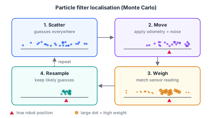
Each cycle, guesses that disagree with the sensors die out and guesses that agree multiply.
- Scatter particles across the map, because at first the robot could be anywhere.
- Move every particle by the odometry reading, plus a little random noise.
- Weigh each particle: if the robot were there, how likely is the actual sensor reading?
- Resample: draw a new set of particles, picking high-weight ones more often.
- Repeat. The cloud shrinks onto the true pose.
Here is a robot in a 20 m corridor that can only sense "door" or "wall" beside it, and is wrong 5 percent of the time. It does not know where it starts.
import numpy as np
rng = np.random.default_rng(2)

DOORS = np.array([2.0, 5.0, 6.0, 13.0, 17.0])          # door centres, metres
at_door = lambda x: np.min(np.abs(np.subtract.outer(x, DOORS)), axis=-1) < 0.5

N, true_x = 1000, 0.0
particles = rng.uniform(0, 20, N)                      # no idea where we are
for step in range(1, 13):
    true_x += 1.0                                      # robot moves 1 m
    particles = particles + 1.0 + rng.normal(0, 0.1, N)
    reading = bool(at_door(np.array([true_x]))[0])
    if rng.random() < 0.05:
        reading = not reading                          # sensor mistake
    weights = np.where(at_door(particles) == reading, 0.95, 0.05)
    weights[particles > 20] = 0                        # outside the corridor
    weights /= weights.sum()
    particles = rng.choice(particles, N, p=weights)    # resample
    print(f"step {step}: true x={true_x:4.1f}  sensed {'door' if reading else 'wall'}  "
          f"estimate={particles.mean():5.2f}  spread={particles.std():4.2f} m")
For the first few steps the spread stays above 5 m, because several places in the corridor look alike. The pair of doors at 5 and 6 m is distinctive, so the cloud tightens there, and a long stretch of plain wall then rules out the spots near 13 and 17 m.
By step 10 the spread is under 30 cm and the estimate tracks the true position. The false "door" at step 4 did not derail it, because one bad reading only lowers weights; it does not delete every good guess.
In ROS 2, Nav2's AMCL (adaptive Monte Carlo localisation) does exactly this in 2D, weighting particles by comparing lidar scans with the saved map.
Quick check
What does resampling do in a particle filter?
Resampling draws a new particle set in proportion to the weights, so guesses that match the sensors multiply and poor guesses disappear.
What is SLAM?
Localisation needs a map. Building a map needs to know where you are. SLAM solves both at the same time, which is why it is often called a chicken-and-egg problem.
SLAM (simultaneous localisation and mapping) is the technique by which a robot builds a map of an unknown environment while continuously estimating its own pose within that map.
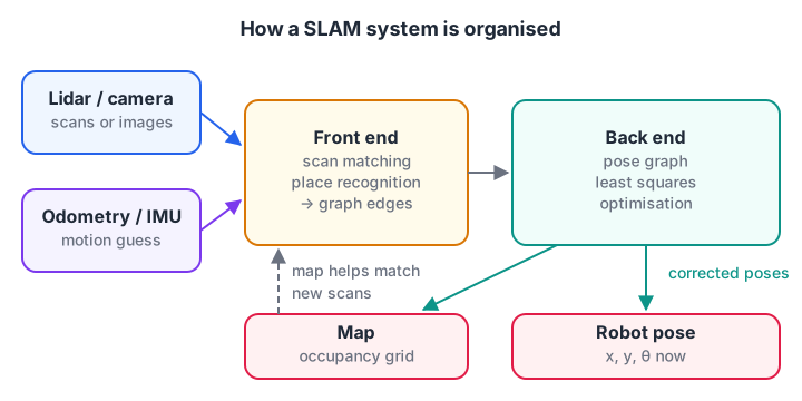
The front end turns raw data into constraints; the back end finds the trajectory that satisfies them best.
A modern SLAM system has two halves. The front end looks at sensor data: it aligns each new lidar scan with recent ones to estimate motion, and it watches for places seen before.
The back end keeps a pose graph, where every node is a robot pose and every edge is a measured relation between two poses, and adjusts the poses so all the edges agree as well as possible.
How does loop closure fix drift?
Odometry edges are each a little wrong, and the errors add up, exactly as you saw in wheel encoders and odometry. A loop closure edge says "pose 16 is at the same place as pose 0".
The back end then solves a least squares problem: find the poses that best fit all the odometry edges and the loop closure together. The error gets spread back over the whole loop instead of piling up at the end. This block drives a 4 m square with drifting odometry, then solves the pose graph with numpy.
import numpy as np
rng = np.random.default_rng(1)

moves = [(1, 0)] * 4 + [(0, 1)] * 4 + [(-1, 0)] * 4 + [(0, -1)] * 4   # a 4 m square
true = np.vstack([[0, 0], np.cumsum(moves, axis=0)]).astype(float)
odom = np.array(moves) + np.array([0.03, 0.05]) + rng.normal(0, 0.02, (16, 2))
dead_reckoned = np.vstack([[0, 0], np.cumsum(odom, axis=0)])

n = 17                                          # poses 0..16
rows, rhs, w = [], [], []
def edge(i, j, meas, sigma):                    # constraint: pose j - pose i = meas
    r = np.zeros(n); r[j], r[i] = 1, -1
    rows.append(r); rhs.append(meas); w.append(1 / sigma)
for k in range(16):
    edge(k, k + 1, odom[k], 0.05)               # odometry edges
edge(0, 16, np.zeros(2), 0.01)                  # loop closure: back at the start
anchor = np.zeros(n); anchor[0] = 1
rows.append(anchor); rhs.append(np.zeros(2)); w.append(100)   # fix pose 0 at origin

A = np.array(rows) * np.array(w)[:, None]
b = np.array(rhs) * np.array(w)[:, None]
optimised = np.linalg.lstsq(A, b, rcond=None)[0]

for name, est in (("odometry only", dead_reckoned), ("after loop closure", optimised)):
    err = np.linalg.norm(est - true, axis=1)
    print(f"{name:19} end error {err[-1]:.3f} m   worst pose error {err.max():.3f} m")
Odometry alone ends about 0.9 m from where it started. After loop closure, the end error drops to a few millimetres and the worst error anywhere on the loop falls to about 6 cm. Real SLAM back ends do the same with headings included, which makes the problem non-linear and needs iterative solvers.
Quick check
Why is loop closure so important in SLAM?
Recognising a previously visited place ties the end of the trajectory to its start, and optimisation spreads the correction across every pose.
How is the map built? Occupancy grids
Once the poses are known, building the map is straightforward. Each lidar beam travels from the robot to an obstacle. Cells along the beam are probably free, and the cell where it stops is probably occupied.
Robots store each cell as log-odds, a number that grows with every "occupied" vote and shrinks with every "free" vote, which handles noisy readings gracefully.
import math

CELL, N = 0.5, 10                      # 0.5 m cells along one lidar beam
L_FREE, L_OCC = -0.4, 0.85             # log-odds votes
logodds = [0.0] * N                    # 0.0 means 50% unknown

def update(distance):
    hit = int(distance / CELL)
    for i in range(min(hit, N)):
        logodds[i] += L_FREE           # beam passed through: free
    if hit < N:
        logodds[hit] += L_OCC          # beam stopped here: occupied

for d in (3.2, 3.1, 3.3, 1.2, 3.2):    # the 1.2 m reading is a passing person
    update(d)
prob = [1 - 1 / (1 + math.exp(l)) for l in logodds]
print("cell:  " + " ".join(f"{i * CELL:4.1f}" for i in range(N)))
print("P(occ):" + " ".join(f"{p:4.2f}" for p in prob))
The cell at 3.0 m ends up 97 percent occupied and the cells before it lean clearly towards free. The one-off reading at 1.2 m, a person walking past, leaves its cell at only 32 percent, still on the free side, because four other beams passed straight through it.
Types of SLAM
| Approach | Sensor | Idea | Common ROS 2 tools |
|---|---|---|---|
| 2D lidar SLAM | Planar lidar | Scan matching plus pose graph | slam_toolbox, Cartographer |
| Visual SLAM | Camera (mono, stereo, depth) | Track image features across frames | ORB-SLAM3, RTAB-Map |
| Lidar-inertial or visual-inertial | 3D lidar or camera with IMU | Fuse an IMU for fast motion | Many research packages |
| EKF-SLAM | Any landmark sensor | Landmarks in a Kalman filter state | Mostly teaching and small maps |
Running SLAM in ROS 2
With a robot or simulation publishing /scan, /odom and the TF transforms, building and saving a map in ROS 2 Jazzy takes three commands. The Gazebo simulation lesson shows how to get a simulated robot publishing these.
# Terminal 1: start your robot or simulation (publishes /scan, /odom, TF)
# Terminal 2: build the map while you drive
ros2 launch slam_toolbox online_async_launch.py use_sim_time:=true
# Terminal 3: once the map looks complete, save it
ros2 run nav2_map_server map_saver_cli -f ~/maps/lab_map
The saver writes an image (lab_map.pgm) and a description file (lab_map.yaml). Nav2 then loads that map, localises on it with AMCL, and plans routes with the algorithms from path planning with A* and Dijkstra.
Common localisation and SLAM mistakes
- Driving too fast while mapping. Scan matching fails when consecutive scans barely overlap. Drive slowly and turn gently.
- Never closing a loop. Without returning to known places, SLAM is just odometry with extra steps.
- Wrong TF frames. If the lidar's position on the robot is set wrongly, every scan lands in the wrong place.
- Too few particles. Global localisation in a big building needs thousands of particles; tracking needs far fewer.
- Mapping a changing scene. People and moved furniture leave ghost obstacles. Map when the space is quiet.
Key takeaways
- Localisation estimates the robot's pose on a map; SLAM builds the map at the same time.
- Particle filters handle global localisation by keeping many guesses and resampling.
- SLAM front ends match sensor data; back ends optimise a pose graph.
- Loop closure turns accumulated drift into a small error spread over the whole path.
- Occupancy grids store log-odds per cell, built from lidar beams once poses are known.
- In ROS 2, map with slam_toolbox, save with map_saver_cli, localise with AMCL in Nav2.
FAQ
What is the difference between localisation and SLAM?
Localisation assumes the map already exists and only estimates where the robot is on it. SLAM has no map at the start, so it estimates the robot's pose and builds the map simultaneously. Robots often run SLAM once to make a map, then switch to plain localisation for daily work.
Can SLAM work with just a camera?
Yes. Visual SLAM uses camera images, tracking distinctive features between frames to estimate motion and build a map. A single camera cannot measure scale on its own, so many systems add a depth camera, a second camera or an IMU. Lidar SLAM is usually easier to get working on a first indoor robot.
Do I need a lidar to learn SLAM?
Not to start. You can learn the ideas in Python simulations like the ones above, then run slam_toolbox on a simulated robot with a simulated lidar in Gazebo. Affordable 2D lidars are available when you want to try it on real hardware.
What is AMCL in ROS 2?
AMCL stands for adaptive Monte Carlo localisation. It is the particle filter localiser in the Nav2 stack. It compares laser scans with a saved map to estimate the robot's pose, and adapts the number of particles to how uncertain it is.
Where can I learn ROS 2 and robot navigation in Indore?
You can learn the foundations through a robotics course at Debugshala that goes up to ROS 2, at its Old Palasia campus.
It covers Python for robotics, sensors, motors, Raspberry Pi with a camera and ROS 2 basics (nodes and topics), ending with a final robot project, taught in English and Hindi with a free demo class. You can also take a reasoning quiz on Debugshala Test.
From the team behind this site
Go further with the Robotics Course at Debugshala
These tutorials are written by Debugshala, a training and placement institute at Old Palasia, Indore. The classroom course adds live mentoring, real projects and interview preparation.
- Offline classes at Old Palasia, Indore
- Free demo class before you pay
- Non-IT, fresher and year-gap friendly
- Placement assistance
700+ students placed · 200+ hiring partners · 4.9★ Google rating
