

Robot Kinematics: Forward and Inverse Kinematics in Python
Robot kinematics for beginners: forward kinematics of a 2-link arm, transformation matrices, inverse kinematics with the law of cosines and Jacobian IK.
Imagine you are reaching for a steel tumbler on the top kitchen shelf. You do not think "shoulder 40 degrees, elbow 65 degrees". You think "hand, go there", and your brain works out the joint angles for you.
Now flip it. Close your eyes while a friend bends your arm into some position. You can still say roughly where your hand is, because you can feel your shoulder and elbow angles and you know how long your arm is.
Those are the two halves of robot kinematics. One direction is easy and exact. The other is the one robots actually need, and it is harder.
What is robot kinematics?
Map the kitchen onto a robot arm. Your upper arm and forearm are the robot's links. Your shoulder and elbow are its joints. Your hand is the end effector, such as a gripper. Feeling your joint angles and knowing where your hand is is forward kinematics. Picking angles to reach the tumbler is inverse kinematics.
Robot kinematics is the study of how a robot's joint positions determine the position and orientation of its links and end effector, without considering the forces that cause the motion.
Forces and torques belong to dynamics, a separate topic. Kinematics is pure geometry.
| Forward kinematics (FK) | Inverse kinematics (IK) | |
|---|---|---|
| Input | Joint angles | Desired end-effector position (and orientation) |
| Output | End-effector position | Joint angles |
| Number of answers | Exactly one | Zero, one, two or infinitely many |
| Difficulty | Straightforward | Harder, often iterative |
| Used for | Displaying the robot, checking reach, simulation | Commanding the arm to pick, place or follow a path |
Joints, links and degrees of freedom
A revolute joint rotates, like a servo or an elbow. A prismatic joint slides in a straight line, like a 3D printer's axis. Each independent joint adds one degree of freedom (DOF).
A hobby arm with base, shoulder and elbow servos has 3 DOF, enough to reach points in 3D space but not to choose the gripper's angle freely. Industrial arms usually have 6 DOF: three to reach a position and three to set orientation. The servo motors lesson covers the hardware that usually drives these joints on small arms.
This article uses a 2-link planar arm: two revolute joints moving in a flat plane. It is small enough to understand completely, and the same ideas scale to bigger arms.
How does forward kinematics work?
Put the shoulder at the origin. Link 1 has length L1 and makes angle θ1 with the x-axis. Link 2 has length L2 and bends by θ2 relative to link 1. The elbow and the hand positions follow from basic trigonometry.
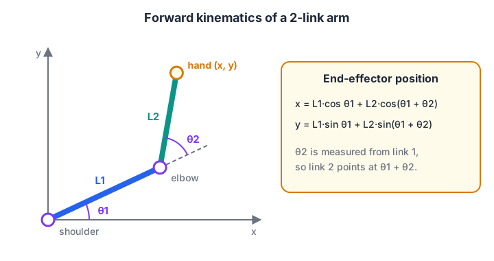
Each link adds its own length in the direction set by the sum of all the angles before it.
- elbow: x = L1·cos θ1, y = L1·sin θ1
- hand: x = L1·cos θ1 + L2·cos(θ1 + θ2), y = L1·sin θ1 + L2·sin(θ1 + θ2)
The key detail is θ1 + θ2. Because θ2 is measured relative to link 1, the second link's absolute direction is the sum of both angles.
import math

L1, L2 = 0.12, 0.10                 # metres, a small desktop arm

def fk(t1_deg, t2_deg):
    t1, t2 = math.radians(t1_deg), math.radians(t2_deg)
    ex, ey = L1 * math.cos(t1), L1 * math.sin(t1)
    hx = ex + L2 * math.cos(t1 + t2)
    hy = ey + L2 * math.sin(t1 + t2)
    return (ex, ey), (hx, hy)

for angles in [(0, 0), (90, 0), (45, 45), (30, 90), (60, -60)]:
    (ex, ey), (hx, hy) = fk(*angles)
    print(f"theta={angles}  elbow=({ex:6.3f}, {ey:6.3f})  hand=({hx:6.3f}, {hy:6.3f}) m")
Check the first row by eye: with both angles zero the arm lies flat along x, and the hand is at 0.12 + 0.10 = 0.22 m. That kind of sanity check catches most sign mistakes.
Forward kinematics with transformation matrices
Trigonometry gets messy beyond two or three joints. The standard method instead gives each joint a small homogeneous transformation matrix that rotates by the joint angle and then moves along the link. Multiplying the matrices in order gives the pose of every link.
In 2D each matrix is 3×3: a rotation block plus a translation column. In 3D they are 4×4. Industrial arms describe the chain with Denavit–Hartenberg (DH) parameters, and ROS 2 describes it in a URDF file, covered in describing a robot with URDF.
import numpy as np

def joint(theta_deg, length):
    t = np.radians(theta_deg)
    c, s = np.cos(t), np.sin(t)
    return np.array([[c, -s, length * c],     # rotate by theta, then move
                     [s,  c, length * s],     # along the rotated link
                     [0,  0, 1.0]])

# 3-joint planar arm: two links plus a 4 cm gripper
chain = [(30, 0.12), (90, 0.10), (-45, 0.04)]
T = np.eye(3)
for i, (theta, length) in enumerate(chain, start=1):
    T = T @ joint(theta, length)
    heading = np.degrees(np.arctan2(T[1, 0], T[0, 0]))
    print(f"after joint {i}: x={T[0, 2]:.4f} m  y={T[1, 2]:.4f} m  heading={heading:.0f} deg")
The first two rows match the trigonometric version for angles (30, 90). The third joint adds a gripper whose final heading is 30 + 90 − 45 = 75 degrees. The matrix version also gives you orientation for free, which the plain formula did not.
How does inverse kinematics work for a 2-link arm?
Now the hard direction: given a target (x, y), find θ1 and θ2. For two links there is a neat closed-form answer from the law of cosines.
- Distance from shoulder to target: r² = x² + y².
- Reachability check: the target is reachable only if |L1 − L2| ≤ r ≤ L1 + L2.
- Elbow angle: cos θ2 = (r² − L1² − L2²) / (2·L1·L2). Take θ2 = ±acos of that value.
- Shoulder angle: θ1 = atan2(y, x) − atan2(L2·sin θ2, L1 + L2·cos θ2).
- Verify by running forward kinematics on the answer.
The ± in step 3 is not a typo. Most targets can be reached two ways, elbow up or elbow down.
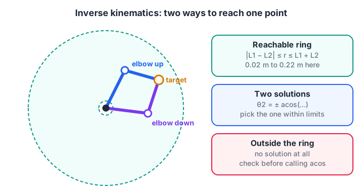
Every reachable point inside the ring has two arm shapes; points outside the ring have none.
import math

L1, L2 = 0.12, 0.10

def ik(x, y, elbow_up=True):
    r2 = x * x + y * y
    c2 = (r2 - L1**2 - L2**2) / (2 * L1 * L2)
    if not -1 <= c2 <= 1:
        return None                                  # outside the workspace
    t2 = math.acos(c2) * (-1 if elbow_up else 1)
    t1 = math.atan2(y, x) - math.atan2(L2 * math.sin(t2), L1 + L2 * math.cos(t2))
    return math.degrees(t1), math.degrees(t2)

def fk(t1, t2):
    t1, t2 = math.radians(t1), math.radians(t2)
    return (L1 * math.cos(t1) + L2 * math.cos(t1 + t2),
            L1 * math.sin(t1) + L2 * math.sin(t1 + t2))

for target in [(0.15, 0.08), (0.05, 0.18), (0.30, 0.0)]:
    for up in (True, False):
        sol = ik(*target, elbow_up=up)
        if sol is None:
            print(f"target {target}: unreachable (max reach {L1 + L2:.2f} m)"); break
        x, y = fk(*sol)
        print(f"target {target} elbow {'up  ' if up else 'down'}: "
              f"theta1={sol[0]:6.1f}  theta2={sol[1]:6.1f}  check=({x:.3f}, {y:.3f})")
Both solutions land exactly on the target, and the third target is rejected because it is beyond the 0.22 m reach. In a real arm you would pick the solution that keeps the servos within their limits and avoids hitting the table.
Quick check
A 2-link arm has L1 = 0.12 m and L2 = 0.10 m. Which target distance from the shoulder is unreachable?
Reachable distances lie between |L1 − L2| = 0.02 m and L1 + L2 = 0.22 m. A target 0.25 m away is outside the workspace.
Quick check
Why does inverse kinematics of a 2-link arm usually give two solutions?
The elbow angle comes from acos, which gives plus and minus solutions. Both shapes put the hand on the same target.
Numerical inverse kinematics with the Jacobian
Closed-form IK exists for many common arm designs, but not all of them, and it gets painful with 6 or 7 joints. The general approach is iterative: start from the current angles, see how far the hand is from the target, nudge the angles, and repeat.
The Jacobian is the matrix that says how much the hand moves when each joint moves a tiny bit.
The damped least squares method uses it to compute a safe nudge, and the damping term keeps the arm from making wild jumps near awkward poses. The same kind of matrix of derivatives is what linearises the extended Kalman filter from the previous lesson.
import numpy as np

L1, L2 = 0.12, 0.10
def fk(q):
    return np.array([L1*np.cos(q[0]) + L2*np.cos(q[0]+q[1]),
                     L1*np.sin(q[0]) + L2*np.sin(q[0]+q[1])])
def jacobian(q):
    s1, c1 = np.sin(q[0]), np.cos(q[0]); s12, c12 = np.sin(q[0]+q[1]), np.cos(q[0]+q[1])
    return np.array([[-L1*s1 - L2*s12, -L2*s12],
                     [ L1*c1 + L2*c12,  L2*c12]])

target, q, lam = np.array([0.05, 0.18]), np.radians([10.0, 20.0]), 0.03
print(f"start : error={np.linalg.norm(target - fk(q)) * 1000:7.3f} mm")
for it in range(1, 30):
    err = target - fk(q)
    if np.linalg.norm(err) < 1e-5:
        break
    J = jacobian(q)
    dq = J.T @ np.linalg.solve(J @ J.T + lam**2 * np.eye(2), err)
    q = q + dq
    print(f"iter {it}: theta=({np.degrees(q[0]):6.1f}, {np.degrees(q[1]):6.1f}) deg  "
          f"error={np.linalg.norm(target - fk(q)) * 1000:7.3f} mm")
The error shrinks from about 190 mm to a few thousandths of a millimetre in eight iterations, and the answer matches the elbow-down solution from the closed-form version. Libraries such as MoveIt 2 in ROS 2 use more refined versions of this idea for full 6-DOF arms, adding joint limits and collision checks.
From joint angles to real servos
Kinematics gives angles in the maths convention. Your servo expects a pulse or a 0 to 180 degree command, with its own zero position. You need a small mapping layer:
- Offset: if the servo's 90 degree position points the link straight up, then servo command = θ + 90 for that joint.
- Direction: a servo mounted the other way round needs servo command = 90 − θ.
- Limits: reject or clamp any IK answer outside the servo's safe range before sending it.
Measure each joint's real offset once with a protractor and keep the values in one place in your code. The full build, including wiring and a pick-and-place routine, is in the robotic arm project.
Common kinematics mistakes
- Mixing degrees and radians. Python's
math.cosexpects radians. - Using
ataninstead ofatan2. Plainatan(y / x)loses the quadrant and fails when x is 0. - Forgetting θ1 + θ2. The second link's direction is the sum of the angles, not θ2 alone.
- Ignoring unreachable targets. Without the reachability check,
acosraises a math domain error. - Not verifying IK with FK. Always run the answer through forward kinematics before moving hardware.
Key takeaways
- Kinematics relates joint positions to end-effector position, ignoring forces.
- Forward kinematics is exact and unique: add each link in the direction of the summed angles.
- Transformation matrices chain joints cleanly and also give orientation.
- Inverse kinematics can have two, many or no solutions; check reachability first.
- Use closed-form IK for small arms and Jacobian-based iteration for larger ones, then map angles to servo commands.
FAQ
What is the difference between forward and inverse kinematics?
Forward kinematics calculates where the end effector is from known joint angles, and always has one answer. Inverse kinematics calculates the joint angles needed to reach a desired position, and may have several answers or none. Robots use FK to know where they are and IK to decide how to move.
What maths do I need for robot kinematics?
You need trigonometry (sine, cosine, atan2 and the law of cosines) for planar arms, and basic matrix multiplication for transformation matrices. For numerical IK you also use the Jacobian, which is a matrix of derivatives. Plain Python and numpy are enough to practise all of it.
Does a mobile robot have kinematics too?
Yes. A wheeled robot's kinematics relates wheel speeds to how the robot body moves and turns. For a two-wheeled robot this is called differential drive kinematics, and it is the subject of the next lesson on differential drive robots.
What is a singularity in robot kinematics?
A singularity is a pose where the arm loses the ability to move its hand in some direction, such as when it is fully stretched out. Near a singularity, IK can demand huge joint speeds. Damped least squares and joint limits keep the robot well-behaved there.
Where can I build a robotic arm and learn kinematics in Indore?
Debugshala's robotics training with Python and servos is project-based and runs at the Old Palasia campus in English and Hindi. It covers Python for robotics, servos and motor drivers, Arduino and ESP32, ROS 2 basics and a final robot project, with a free demo class first. For trigonometry-style warm-ups, solve aptitude questions on Debugshala Test.
From the team behind this site
Go further with the Robotics Course at Debugshala
These tutorials are written by Debugshala, a training and placement institute at Old Palasia, Indore. The classroom course adds live mentoring, real projects and interview preparation.
- Offline classes at Old Palasia, Indore
- Free demo class before you pay
- Non-IT, fresher and year-gap friendly
- Placement assistance
700+ students placed · 200+ hiring partners · 4.9★ Google rating
