

A* Path Planning vs Dijkstra: Grid Robot Navigation in Python
Learn robot path planning with A* and Dijkstra: occupancy grids, f = g + h, heuristics, step-by-step Python traces and how Nav2 plans routes in ROS 2.
Imagine you need to walk from Rajwada to a friend's house near Vijay Nagar, and someone has closed several lanes for a wedding procession. One way to plan is to explore every street around you, a little further each time, like ripples spreading in a pond, until a ripple touches your friend's door.
That works, and it always finds the shortest route. But it also wastes time exploring lanes heading towards Rau, completely the wrong way.
A smarter walker keeps a sense of direction: "Vijay Nagar is north-east, so try those streets first." You still check other options when a lane is blocked, but you stop wandering away from the goal. Those two walkers are Dijkstra's algorithm and A*.
What is path planning in robotics?
Map the walk onto a robot. The city streets are a graph: places are nodes, and streets are edges with a length or cost. The closed lanes are obstacles. The ripple walker is Dijkstra's algorithm. The walker with a sense of direction is A*, and that sense of direction is called a heuristic.
Path planning is the process of computing a sequence of positions that takes a robot from a start to a goal while avoiding obstacles and minimising a cost such as distance or time.
Robots usually plan at two levels. A global planner finds the whole route on a map, which is what this article covers. A local planner or controller then follows it while dodging things that move, much like the go-to-goal controller in the differential drive robots lesson.
How do robots represent the map?
Most mobile robots use an occupancy grid: the floor divided into small square cells, each marked free, occupied or unknown. A 5 cm grid of a 10 m × 10 m room has 200 × 200 = 40,000 cells.
Each free cell is a node, linked to its neighbours. The map itself usually comes from SLAM, the next lesson in this series.
- 4-connected: move up, down, left or right, each costing 1.
- 8-connected: diagonals too, costing √2 ≈ 1.414, which gives smoother, shorter paths.
Other robots plan on a waypoint graph instead: a few named points, like loading docks and aisle ends in a warehouse, joined by known corridors. The same algorithms work on both.
How does Dijkstra's algorithm work?
Dijkstra's algorithm keeps a priority queue of places to visit, always taking out the one with the smallest cost from the start, called g.
- Set the start's cost to 0 and every other node's to infinity. Put the start in the queue.
- Pop the node with the lowest g. If it is the goal, stop.
- For each neighbour, compute g of the current node plus the edge cost. If this beats the neighbour's best so far, record it and remember the current node as its parent.
- Push improved neighbours into the queue and repeat from step 2.
- Walk back through the parents from the goal to read off the path.
Here it is on a waypoint graph of a small warehouse, using Python's heapq module as the priority queue.
import heapq

GRAPH = {  # corridor lengths in metres
    "dock":    {"aisle1": 4, "aisle2": 7},
    "aisle1":  {"dock": 4, "aisle2": 2, "cold": 9},
    "aisle2":  {"dock": 7, "aisle1": 2, "packing": 3},
    "packing": {"aisle2": 3, "cold": 2, "office": 6},
    "cold":    {"aisle1": 9, "packing": 2, "office": 3},
    "office":  {"packing": 6, "cold": 3},
}

def dijkstra(start, goal):
    queue, best, parent = [(0, start)], {start: 0}, {start: None}
    while queue:
        g, node = heapq.heappop(queue)
        if g > best[node]:
            continue                        # stale entry, a cheaper one was found
        print(f"  visit {node:8} cost so far {g}")
        if node == goal:
            break
        for nb, length in GRAPH[node].items():
            if g + length < best.get(nb, float("inf")):
                best[nb], parent[nb] = g + length, node
                heapq.heappush(queue, (g + length, nb))
    path, node = [], goal
    while node:
        path.append(node); node = parent[node]
    return path[::-1], best[goal]
path, cost = dijkstra("dock", "office")
print("shortest route:", " -> ".join(path), f"({cost} m)")
Notice the order of visits: always the closest unvisited node first. The route with the fewest corridors, dock → aisle1 → cold → office, costs 16 m. Dijkstra finds a 14 m route that uses more corridors, each of them short.
How does the A* algorithm work?
A* is Dijkstra with a sense of direction. For each node it adds a heuristic h, an estimate of the cost still to go, and it pops nodes in order of f = g + h instead of g alone.
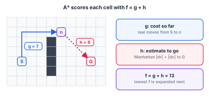
g looks back at the cost already paid; h looks ahead at the cost still expected.
Nodes that lie in the general direction of the goal get a small f and are expanded early. Nodes heading away get a large f and may never be expanded at all. If h is always 0, A* becomes exactly Dijkstra.
Choosing the heuristic
| Heuristic | Formula (dx, dy = distance to goal in cells) | Use with | Optimal? |
|---|---|---|---|
| Zero | 0 | Any graph | Yes, this is Dijkstra |
| Manhattan | dx + dy | 4-connected grid | Yes |
| Octile | max(dx, dy) + 0.414 × min(dx, dy) | 8-connected grid | Yes |
| Euclidean | √(dx² + dy²) | Any-angle or 8-connected | Yes, but expands more than octile |
| Weighted, e.g. 2 × Manhattan | 2(dx + dy) | When speed matters more than the perfect path | Not guaranteed |
The rule behind the "Optimal?" column: a heuristic is admissible if it never overestimates the true remaining cost. Admissible heuristics guarantee A* returns a shortest path.
Watching A* decide, step by step
This tiny 4 × 5 grid has a wall in the middle column. The block prints every cell A* pops, with its g, h and f, so you can see why each choice is made.
import heapq

GRID = ["S.#..",
        "..#..",
        "....G",
        "....."]
start, goal = (0, 0), (2, 4)
h = lambda c: abs(c[0] - goal[0]) + abs(c[1] - goal[1])     # Manhattan

heap, best, done = [(h(start), h(start), 0, start)], {start: 0}, set()
while heap:
    f, hc, g, cell = heapq.heappop(heap)
    if cell in done:
        continue
    done.add(cell)
    print(f"pop {cell}: g={g} h={hc} f={f}   open list size {len(heap)}")
    if cell == goal:
        break
    r, c = cell
    for nr, nc in ((r + 1, c), (r - 1, c), (r, c + 1), (r, c - 1)):
        if 0 <= nr < 4 and 0 <= nc < 5 and GRID[nr][nc] != "#":
            if g + 1 < best.get((nr, nc), 99):
                best[(nr, nc)] = g + 1
                heapq.heappush(heap, (g + 1 + h((nr, nc)), h((nr, nc)), g + 1, (nr, nc)))
print(f"goal reached with cost {best[goal]} after expanding {len(done)} of 18 free cells")
Every popped cell has f = 6, the true shortest cost. A* walks straight around the wall without touching the cells in the bottom row or the top right corner. Ties are broken by preferring the smaller h, which pushes the search towards the goal.
Quick check
What happens if you set the A* heuristic to zero for every cell?
With h = 0, f equals g, so nodes are ordered only by cost so far, which is Dijkstra's algorithm.
A* vs Dijkstra on a real grid
Now compare the two on a bigger map with a wall between start and goal. Both use the same code; the only difference is whether h is switched on.
import heapq

GRID = ["....................", "....................", ".........#..........",
        ".........#..........", "..S......#.......G..", ".........#..........",
        "......####..........", "....................", "...................."]
R, C = len(GRID), len(GRID[0])
START, GOAL = (4, 2), (4, 17)
def plan(use_h):
    h = lambda p: (abs(p[0] - GOAL[0]) + abs(p[1] - GOAL[1])) if use_h else 0
    heap, closed = [(h(START), h(START), 0, START)], set()
    g, parent = {START: 0}, {START: None}
    while heap:
        _, _, cost, cell = heapq.heappop(heap)
        if cell in closed: continue
        closed.add(cell)
        if cell == GOAL: break
        r, c = cell
        for nb in ((r + 1, c), (r - 1, c), (r, c + 1), (r, c - 1)):
            free = 0 <= nb[0] < R and 0 <= nb[1] < C and GRID[nb[0]][nb[1]] != "#"
            if free and cost + 1 < g.get(nb, 1e9):
                g[nb], parent[nb] = cost + 1, cell
                heapq.heappush(heap, (cost + 1 + h(nb), h(nb), cost + 1, nb))
    path, cell = set(), GOAL
    while cell: path.add(cell); cell = parent[cell]
    return path, closed
for name, use_h in (("Dijkstra", False), ("A*", True)):
    path, closed = plan(use_h)
    print(f"{name}: path length {len(path) - 1} moves, cells expanded {len(closed)} of 172")
    for r in range(R):
        print("  " + "".join(GRID[r][c] if GRID[r][c] in "SG#" else "*" if (r, c) in path
              else "o" if (r, c) in closed else "." for c in range(C)))
Both find a 21-move path, but Dijkstra expands 165 cells, almost the whole map, while A* expands 49. On a 40,000-cell office map, that difference is what lets a robot replan several times a second on a small computer.
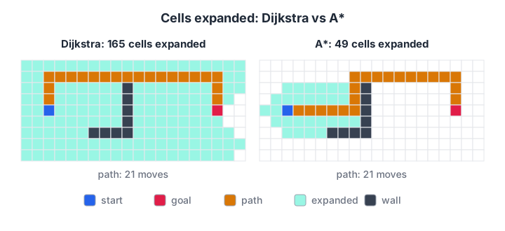
Shaded cells were expanded. Same path cost, roughly a third of the work for A.*
| Dijkstra | A* | |
|---|---|---|
| Orders nodes by | g, cost so far | f = g + h |
| Needs a goal position? | No, can find paths to every node at once | Yes, for the heuristic |
| Finds shortest path? | Always | If h is admissible |
| Cells expanded | Many, in all directions | Far fewer, biased to the goal |
| Best for | Distance maps, many goals, unknown goal location | One start, one goal, known map |
Making planned paths work on a real robot
A path through grid cells is not yet something a robot can drive. Real planners add a few steps:
- Inflate obstacles. Grow every obstacle by the robot's radius plus a safety margin, so the planner can treat the robot as a point.
- Plan with A* on the inflated grid, usually 8-connected with the octile heuristic.
- Smooth the path to remove zig-zags along the grid.
- Follow it with a controller that tracks points along the path, and replan when the map changes.
In ROS 2, the Nav2 navigation stack does all of this. Its NavFn planner runs Dijkstra or A* on a costmap, and the Smac planner family adds variants such as Hybrid-A* for car-like robots. The ROS 2 navigation with Nav2 lesson shows how to configure them.
For robot arms and high-dimensional problems, grids explode in size, so planners use sampling methods such as RRT instead of A*.
Common path planning mistakes
- Planning without inflation. The path hugs walls so tightly that the real robot clips corners.
- Using a heuristic that overestimates. For example, Euclidean distance scaled up, or Manhattan on an 8-connected grid. The path is no longer guaranteed to be the shortest.
- Forgetting diagonal costs. Charging 1 for a diagonal makes zig-zags look as cheap as straight lines.
- Not marking visited cells. Without a closed set, the same cell is expanded again and again.
- Planning on a map that is out of date. Replan regularly, or the robot drives into a newly placed box.
Quick check
Quick check
In A*, a cell has g = 7 and h = 5. What is its f value?
f = g + h = 7 + 5 = 12. A* expands the open cell with the lowest f next.
Key takeaways
- Path planning finds a collision-free, low-cost route on a grid or graph.
- Dijkstra expands by cost so far and always finds the shortest path, but searches in every direction.
- A* orders nodes by f = g + h and searches towards the goal, expanding far fewer cells.
- Keep the heuristic admissible: Manhattan for 4-connected grids, octile for 8-connected.
- Inflate obstacles, smooth the path and replan, as Nav2 does in ROS 2.
FAQ
Is A* always better than Dijkstra?
For a single start and goal on a known map, A* is usually much faster and finds an equally short path. Dijkstra is better when you want the distance to every node, have many possible goals, or cannot estimate the remaining distance. Both are optimal with non-negative edge costs.
What is an admissible heuristic?
An admissible heuristic never overestimates the true cost from a node to the goal. Straight-line distance is admissible for walking robots because no route can be shorter than a straight line. Admissibility guarantees that A* returns a shortest path.
Which path planning algorithm does ROS 2 use?
Nav2 in ROS 2 offers several global planners. NavFn uses Dijkstra or A* on a grid costmap, and the Smac planners provide 2D A*, Hybrid-A* and state lattice planning for robots that cannot turn on the spot. You choose one in the Nav2 parameter file.
Do I need data structures knowledge to learn A*?
You need lists, dictionaries and a priority queue, which Python's built-in heapq module provides. If loops and dictionaries are still new, start with the for loop tutorial and then trace the small A* example above by hand.
Where can I learn robot navigation in Indore?
Debugshala's classroom robotics programme at the Old Palasia campus teaches Python for robotics, obstacle-avoiding robots, Raspberry Pi with a camera and ROS 2 basics, ending with a final robot project. Classes are in English and Hindi with a free demo class. You can also practise algorithm questions on Debugshala Test.
From the team behind this site
Go further with the Robotics Course at Debugshala
These tutorials are written by Debugshala, a training and placement institute at Old Palasia, Indore. The classroom course adds live mentoring, real projects and interview preparation.
- Offline classes at Old Palasia, Indore
- Free demo class before you pay
- Non-IT, fresher and year-gap friendly
- Placement assistance
700+ students placed · 200+ hiring partners · 4.9★ Google rating
