

Kalman Filter Explained: Step-by-Step Python Simulation
The Kalman filter explained with a robot example: predict and update steps, the Kalman gain, a numpy position-velocity tracker and how to tune Q and R.
Imagine you are on a night train from Indore to Bhopal with no phone signal. You know the train runs at about 60 km/h, so after half an hour you guess you have covered 30 km. That is a prediction, and the longer you go without checking, the less sure you are.
Every so often the train passes a kilometre stone, but the window is foggy and you can only half read it. Was that 34 or 31? The stone is evidence, but it is noisy evidence too.
A sensible traveller does not throw away either clue. You nudge your guess towards the stone, more if your guess was shaky, less if the stone was hard to read. That nudge is the whole idea of a Kalman filter.
What is a Kalman filter?
Map the train ride onto a robot. Your guess from speed and time is the prediction from a motion model. The foggy kilometre stone is a measurement from a sensor. How sure you are about each is its variance. And how far you nudge your guess is the Kalman gain.
A Kalman filter is a recursive estimation algorithm that combines a motion model and noisy measurements, weighting each by its uncertainty, to give the best linear estimate of a system's state and how uncertain that estimate is.
"Recursive" means it only keeps the latest estimate and its uncertainty, not the whole history. That makes it light enough for a microcontroller. It is used in GPS receivers, drones, phone orientation, and almost every robot that fuses IMU readings with wheel odometry.
How does a Kalman filter work? Predict and update
Every cycle has two steps, and each changes both the estimate and its uncertainty.
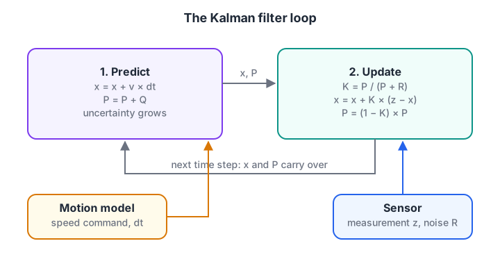
Prediction always makes you less certain; a measurement always makes you more certain.
- Predict. Move the estimate using what you know about motion:
x = x + velocity × dt. Add process noise to the variance:P = P + Q, because the model is never perfect. - Compute the gain.
K = P / (P + R), where R is the sensor's variance. K is always between 0 and 1. - Update. Correct the estimate by a fraction of the surprise:
x = x + K × (z − x), where z is the measurement. The termz − xis called the innovation. - Shrink the uncertainty.
P = (1 − K) × P. - Repeat at the next time step.
This is Bayes' theorem applied to bell curves. The prediction is your prior, the measurement is your evidence, and the update gives the posterior.
Quick check
The prediction has variance 9 and the sensor has variance 1. What is the Kalman gain?
K = P / (P + R) = 9 / 10 = 0.9, so the filter moves 90% of the way towards the measurement because the prediction is far less certain.
Quick check
What happens to the uncertainty P during the predict step?
Predicting forward without new data always adds uncertainty. Only the update step, using a measurement, reduces P.
What does the Kalman gain mean?
The gain is a trust dial. If the prediction is very uncertain (P large), K approaches 1 and the filter mostly believes the sensor. If the sensor is very noisy (R large), K approaches 0 and the filter mostly ignores it.
Take numbers. Your prediction says 10 m with variance 4 (standard deviation 2 m). The sensor reads 12 m with variance 1. Then K = 4 / (4 + 1) = 0.8, the new estimate is 10 + 0.8 × 2 = 11.6 m, and the new variance is 0.2 × 4 = 0.8.
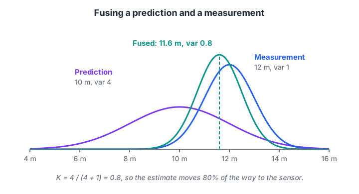
The fused estimate sits closer to the more certain source, and it is narrower than both inputs.
Notice that the final variance, 0.8, is smaller than either input. Combining two independent clues always leaves you more certain than the better clue alone.
A 1D Kalman filter in Python, step by step
Here a small robot drives along a corridor at a commanded 0.5 m/s. Its wheels slip a little, so the prediction drifts. An ultrasonic sensor measures distance from the start wall with about 15 cm of noise. The block prints every number at every step so you can follow the cycle.
import random
random.seed(4)

dt, speed = 0.5, 0.5          # seconds per step, commanded m/s
Q, R = 0.01, 0.15 ** 2        # process variance, sensor variance (m^2)
x, P = 0.0, 1.0               # initial guess and its variance
true = 0.0

print("step  true  predict  P_pred  meas   K     estimate  P")
for step in range(1, 9):
    true += speed * dt * random.uniform(0.85, 1.05)    # wheel slip
    z = true + random.gauss(0, 0.15)                   # noisy sensor
    x, P = x + speed * dt, P + Q                        # predict
    pred, p_pred = x, P
    K = P / (P + R)                                     # gain
    x, P = x + K * (z - x), (1 - K) * P                 # update
    print(f"{step:3d}  {true:5.2f}  {pred:6.2f}  {p_pred:6.3f}  {z:5.2f}  "
          f"{K:.2f}  {x:7.2f}  {P:.4f}")
Watch the K column. On the first step, the initial guess is very uncertain, so K is close to 1 and the filter jumps to the measurement. Within a few steps K settles to a steady value near 0.5, where the uncertainty added by prediction balances the uncertainty removed by each measurement.
Tracking position and velocity with numpy matrices
Real robots track several quantities at once. The same five steps work with matrices: the state becomes a vector, P becomes a covariance matrix, and divisions become matrix inverses.
| Symbol | Meaning | In this example |
|---|---|---|
| x | State vector | [position, velocity] |
| F | State transition (motion model) | position += velocity × dt |
| H | Measurement model | the sensor sees position only |
| Q | Process noise covariance | how much velocity can change unexpectedly |
| R | Measurement noise covariance | sensor variance, 0.2² m² |
| P | Estimate covariance | uncertainty of position and velocity |
The neat part: the sensor only measures position, yet the filter also estimates velocity, because the model links the two.
import numpy as np
rng = np.random.default_rng(0)

dt, n = 0.1, 150
F = np.array([[1, dt], [0, 1]]); H = np.array([[1.0, 0.0]])
Q = np.array([[dt**4 / 4, dt**3 / 2], [dt**3 / 2, dt**2]]) * 0.1 ** 2
R = np.array([[0.2 ** 2]])
x, P = np.zeros((2, 1)), np.eye(2) * 10

true_v = 0.4 + np.cumsum(rng.normal(0, 0.003, n))      # speed wanders slightly
true_p = np.cumsum(true_v * dt)
z = true_p + rng.normal(0, 0.2, n)

est = []
for k in range(n):
    x, P = F @ x, F @ P @ F.T + Q                       # predict
    S = H @ P @ H.T + R
    K = P @ H.T @ np.linalg.inv(S)                      # gain (2x1)
    x = x + K @ (z[k] - H @ x).reshape(1, 1)            # update
    P = (np.eye(2) - K @ H) @ P
    est.append(x.ravel())
est = np.array(est)
rmse = lambda a: np.sqrt(np.mean((a - true_p) ** 2))
print(f"raw sensor RMSE : {rmse(z):.3f} m")
print(f"Kalman RMSE     : {rmse(est[:, 0]):.3f} m")
print(f"final velocity  : estimated {est[-1, 1]:.2f} m/s, true {true_v[-1]:.2f} m/s")
The filter cuts the position error to about a third of the raw sensor error and recovers the speed it was never told, within a few centimetres per second. This is the pattern behind robot_localization in ROS 2, which fuses odometry, IMU and GPS with an extended version of these equations.
How to tune Q and R
R usually comes from the sensor: put the robot still, record 200 readings, and take their variance. Q is a design choice. It says how much the real system can surprise your model between steps.
| If you set... | The filter becomes... | Symptom |
|---|---|---|
| Q too small | Overconfident in the model | Smooth but lags behind real changes |
| Q too large | Twitchy, follows every measurement | Barely smoother than the raw sensor |
| R too small | Trusts a noisy sensor too much | Estimate jitters |
| R too large | Ignores useful measurements | Slow to correct drift |
This block runs the same data with three values of Q to show the trade-off.
import numpy as np
rng = np.random.default_rng(5)

dt, n = 0.1, 150
t = np.arange(n) * dt
true = np.where(t < 7, 0.3 * t, 2.1 + 1.2 * (t - 7))    # robot speeds up at t = 7 s
z = true + rng.normal(0, 0.25, n)
F, H, R = np.array([[1, dt], [0, 1]]), np.array([[1.0, 0]]), 0.25 ** 2

for q in (0.01, 1.0, 100.0):
    Q = q * np.array([[dt**4 / 4, dt**3 / 2], [dt**3 / 2, dt**2]])
    x, P, est = np.zeros(2), np.eye(2), []
    for k in range(n):
        x, P = F @ x, F @ P @ F.T + Q
        K = P @ H.T / (H @ P @ H.T + R)
        x = x + (K * (z[k] - H @ x)).ravel()
        P = (np.eye(2) - K @ H) @ P
        est.append(x[0])
    err = np.array(est) - true
    print(f"q={q:6.2f}  RMSE={np.sqrt(np.mean(err**2)):.3f} m  "
          f"error 1 s after speed-up={err[80]:+.3f} m")
print(f"raw sensor RMSE={np.sqrt(np.mean((z - true)**2)):.3f} m")
The small Q is smooth but falls behind when the robot speeds up. The large Q keeps up but is almost as noisy as the raw sensor. The middle value gives the lowest total error. Start with R from data, then raise or lower Q until the lag and noise both look acceptable.
Extended and unscented Kalman filters
The standard Kalman filter assumes a linear model and bell-shaped noise. Robots that turn break the first assumption, because position depends on the sine and cosine of heading, as you will see in robot kinematics.
| Variant | How it handles non-linear motion | Typical use |
|---|---|---|
| Kalman filter (KF) | Assumes everything is linear | Tracking along a line, simple sensors |
| Extended KF (EKF) | Linearises the model at each step using derivatives (Jacobians) | IMU orientation, wheel plus GPS fusion |
| Unscented KF (UKF) | Pushes a few sample points through the real model | Strongly curved models where EKF struggles |
| Particle filter | Uses hundreds of samples, any noise shape | Localisation on a map, covered in SLAM |
Common Kalman filter mistakes
- Starting with P too small. If the initial guess is wrong but P says you are sure, the filter ignores good measurements for a long time.
- Mixing units. Q, R and the state must use the same units, such as metres and seconds.
- Guessing R. Measure it from still-robot data; it is the easiest number to get right.
- Forgetting that dt changes. If your loop timing varies, rebuild F and Q with the real dt each step.
- Expecting magic with a wrong model. A Kalman filter is only as good as its motion model.
Key takeaways
- A Kalman filter blends a motion prediction with noisy measurements, weighted by their uncertainty.
- Each cycle predicts (uncertainty grows) and updates (uncertainty shrinks).
- The gain K = P / (P + R) is the trust dial between model and sensor.
- With matrices, the filter can estimate quantities you never measure directly, such as velocity.
- Measure R from data, tune Q for the lag-versus-noise trade-off, and use EKF or UKF for turning robots.
FAQ
What is a Kalman filter in simple terms?
A Kalman filter is a method for making the best guess about something you cannot measure perfectly. It predicts where things should be, checks a noisy sensor, and blends the two based on which is more trustworthy, repeating this every time step.
Is the Kalman filter hard to learn?
The one-dimensional version needs only addition, multiplication and division, and you can code it in ten lines. The matrix version needs basic linear algebra such as matrix multiplication and transpose. Most learners understand it best by printing each step, as in this article.
What is the difference between a Kalman filter and a complementary filter?
A complementary filter blends two sensors with fixed weights you choose by hand. A Kalman filter computes the weights every step from modelled uncertainties, can fuse many sensors, and also reports how uncertain its estimate is. The complementary filter is simpler; the Kalman filter is more general.
Where is the Kalman filter used in robotics?
It is used to fuse wheel odometry with IMU data, to estimate drone attitude, to combine GPS with motion sensors in outdoor robots, and to track moving objects seen by cameras. In ROS 2, the robot_localization package provides EKF and UKF nodes for exactly this.
Can I learn sensor fusion and Python for robots in Indore?
Yes. A robotics course in Indore that pairs Python with real sensors runs at Debugshala's Old Palasia campus, covering Python for robotics, Arduino and ESP32, sensors and ROS 2 basics, in English and Hindi, with a free demo class. You can brush up on Python with Debugshala Test quizzes as well.
From the team behind this site
Go further with the Robotics Course at Debugshala
These tutorials are written by Debugshala, a training and placement institute at Old Palasia, Indore. The classroom course adds live mentoring, real projects and interview preparation.
- Offline classes at Old Palasia, Indore
- Free demo class before you pay
- Non-IT, fresher and year-gap friendly
- Placement assistance
700+ students placed · 200+ hiring partners · 4.9★ Google rating
